In my experience, most biologists justify their continued use of Microsoft Excel with the excuse “better the devil you know”. It doesn’t have to be that way!

R is a statistical programming environment that is not only extremely powerful and highly flexible but is also surprisingly easy to use. In this post, I’d like to introduce the absolute beginner to some of the core strengths of R that set it apart from Excel. These are the kinds of commands that we teach in our Data Analysis workshop. In a future post, I’ll do a side-by-side R/Excel comparison.

The only prerequisite is that you have already installed R. R can be downloaded here.

1) Data Management

R stores large data tables in an easily accessible format: A Data Frame

We will consider a built-in data set describing petal and sepal measurements of three species of iris flowers. The measurements are stored as a data frame with the name “iris”. This is equivalent to an Excel file that might be called “iris.xls”. In Excel, to look at the data you would need to open the file, in R we simply write the name of the data frame into the console. Start R and copy and paste the code in the boxes throughout this tutorial.

iris

If the data set is very large we may only want to look at a few lines by using the head() function:

head(iris)

And if we only want to consider data of one species, we can limit our output:

iris[iris$Species =="setosa",]

In Excel, large data tables are very difficult to work with and consume a lot of system resources. Because R doesn’t need to have all the data displayed all the time, it makes working with data much easier.

2) Statistics

It is very straightforward to calculate simple descriptive statistics using our iris data. In Excel, we would click on a free cell and use the mean() function to specify which values we want to calculate the mean for. Although this is convenient because you can easily see exactly which values are included in the mean, it’s also quite cumbersome. In Excel, the analysis of the data exists on the same page as the data itself. If you want to get values for subsets of your data, organisation becomes a problem. In the worst case scenario, you might accidentally change which values are included in your function! So using Excel risks introducing error into your calculations.

In R, the original data frame remains untouched, we can calculate descriptive statistics only for display, or save them using a variable name that we can reuse later on. The equivalent in Excel would be to have a separate file for every group of mean values you calculated. This is not a good idea since you don’t want to clutter your analysis by having lots of files. But in R, since they are only variables holding information, they are very easy to work with.

Let’s look at an example. We can use the tapply() function to sub-divide our “petal width” column according to species and “apply” the mean function to each group.

tapply(iris$Petal.Width,iris$Species,mean)

This function only prints the results to the screen. It is a good start, but not really enough. It would be better to know the mean of each measurement for all three species and to save that information in another variable so we can access it over and over again. In this case we can use the by() function. The by() function I’ve written below sub-divides our data columns 1-4 (containing the measurements) according to the “species” column and takes the column mean using the colMeans() function. This produces a list which is saved as a variable called “mean.list”. To look at the results type “mean.list”:

mean.list <- by(iris[, 1:4], iris$Species, colMeans)
mean.list

The output of a by() functon is a list. Lists are a bit tricky to work with, so to make our analysis easier, we can convert our result into a matrix using the as.matrix() function and save it as a new variable, "mean.ma". Note the difference in structure compared to the list.

mean.ma <- as.matrix(do.call("rbind",mean.list))
mean.ma

3) Data Visualisation

Now that we have our raw data and some descriptive statistics, the next step is to visualise the data. R is extremely flexible when it comes to making graphs.

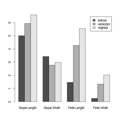
A useful plot would be a representation of our mean values of each measurement for each species. Remember that this is saved in the mean.ma variable that we defined above. First we call the function barplot(). Then we specify the data to use (mean.ma) and set two parameters: "beside" tells the function that we want the bars to appear beside each other, not stacked and "legend" specifies that we want our groups to be labeled using a legend. I have specified the names in the legend using the rownames() function to get the names from the mean.ma matrix.

barplot(mean.ma, beside = TRUE, legend = rownames(mean.ma))

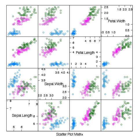
Another very easy option is to plot all variables against each other. This would be a 5x5 scatter plot matrix (splom). This gives us a visual representation of our data and can be done by simply calling the plot() function.

plot(iris)

This is a very rough graph, and we would normally want to adjust things like the main title, variable titles, X- and Y-axis titles, etc. But for this blog post I only want to give an impression of how simple it is to generate such an information-rich plot in R. Generating the equivalent plot in Excel would be much more difficult.

Conclusion

In this post I have showcased each of R's core strengths. Although the examples are relatively simple, they give you an idea of how powerful and flexible R is when working with data. More complicated tasks that are impossible in Excel are simple in R. I have also made use of two key ideas in R:

1) Automatically perform a task using built-in functions

In this example I used a function to calculate the mean, which will be familiar to you from Excel. However, I also used functions to sub-divide the iris data frame and in making the plots. Everything you do in R is structured around functions that carry out clear commands.

2) Reproducible research means you can share your analysis

R's functions make it flexible, but because it is text-based, R is also reproducible. We can save all the commands in a single file and give them to a colleague with the assurance that they will see exactly the same results that we did. There is no chance of accidentally deleting a cell's values, or of accidental mouse clicks introducing intractable errors in our calculations.

Individually, each core strength represents a powerful tool for scientists, once they are mastered. Taken together, its three core strengths make R a powerful alternative to address the limitations and deficiencies of Excel for scientists.

Bonus material:

For the advanced user: We can extend on this plot by using the lattice package. First, we will have to install and activate the lattice graphics package. Then we call the splom() function:

install.packages("lattice", dependencies = TRUE)
library(lattice)
splom(~iris[1:4], groups = iris$Species)

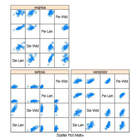
This allows us to very easily differentiate each iris species using colours. But we can also plot a matrix for each species:

splom(~iris[1:4]|Species, data = iris,pscales = 0,varnames = c("Se-Len", "Se-Wid", "Pe-Len","Pe-Wid"))